Framework for cosmography at high redshift

R. Triay ^{[1] [2]}, L. Spinelli and R. Lafaye ^[3]

Université de Provence and Centre de Physique Théorique CNRS, Luminy Case 907, 13288 Marseille cedex 9, France

Accepted 1995 October 12. Received 1995 September 11; in original form 1995 June 29

ABSTRACT

We propose a geometrical framework which is adapted for the investigation of large-scale structures at high redshifts in curved spaces, within the standard world model of the Universe. It is based on the embedding of the comoving space into the 4D metric space, which provides us with a useful algebraic representation of the positions of objects in space. In particular, the interpretation and the calculation of geometrical quantities, such as distances between objects, angles, surfaces and volumes, become obvious. Moreover, elements of cartography provide us with a global view of the Universe which accounts for the curvature. A quasar catalogue is used for observational support. This framework is implemented in a routine called UNIVERSE VIEWER.

Key words: catalogues - cosmology: theory - large-scale structure of Universe.

1 INTRODUCTION

The investigation of the space distribution of large-scale structures (LSSs) and candidate formation theories is one of the main trends in cosmology at present. While Euclidean geometry suffices for describing the spatial distribution of available galaxy catalogues, it is clear that such an analysis when extended to quasar catalogues requires geometry of curved spaces because of the high redshift extent (Triay 1981; Fliche, Souriau & Triay 1982). The aim of the present paper is to provide an understandable framework for cosmography at high redshift. A useful definition of the comoving frame is given in Section 2, where the 'distance between quasars' is clearly defined (these objects are assumed to be permanent sources when their observation relates solely to an event, i.e. the emission of the observed photon in the past). An algebraic representation, which provides us with straightforward calculations of distances, surfaces, volumes, orientations, etc., is given in Section 3. Visual inspections of quasar distributions is a powerful tool for the investigation of LSSs and Section 4 gives a (distortionless) mapping of the Universe. The Burbidge & Hewitt (1993; hereafter BH) quasar catalogue (8000 sources) is used as support of our investigation.

It is clear that such a framework is useless if one limits oneself to a zero curvature space, as predicted by the inflationary scenario (Gliner 1965; Linde 1982). Such a scenario is not so clear cut, however, since the short extragalactic distance scale $H_0=87\pm 7$ km s${}^{-1}$ Mpc${}^{-1}$ (Pierce et al. 1994) suggests a positive curvature (Souriau & Triay 1995). Such an issue reconciles estimated ages for metal-poor Galactic globular clusters $16.5\pm 2$ Gyr (Van den Bergh 1991) with realistic estimates of the density parameter ${\mathrm{\Omega }}_0\sim 0.1$ (which accounts for constraints from the big bang nucleosynthesis or the dynamics of galaxies in clusters).

2 THE WORLD MODEL

The basics of the standard world model are given in Weinberg (1972) and Peebles (1993). The geometry of the space-time $V_4$ is described by an RW metric:

$$\begin{array}{}\text{(1)}& d{s}^4=d{t}^2-a^2(t)d{\sigma }^2\end{array}$$

where $t$ is the cosmic time, $a(t)$ is the (dimensionless) expansion parameter and $d{\sigma }^2$ is the metric element on a homogeneous three-dimensional manifold $V_3$, the comoving space. The sign of its curvature scalar $K$ indicates the type of geometry: Riemannian ($K>0$), Euclidean ($K=0$) or Lobatchevski ($K<0$). Let us denote by $t_0$ the present date (the age of the Universe), and all other variables in similar way.

By defining the expansion parameter so that its present value $a_0=1$, $V_3$ becomes the space-time location from where the CMB can be observed as blackbody radiation at temperature $T_0=2.73\pm 0.03$ K (Wilkinson 1990). If the peculiar velocities are neglected, the redshift $z$ becomes a distance indicator and the quasars have constant coordinates on $V_3$. Hence, the cosmic microwave background (CMB) observed from a quasar at redshift $z$ shows blackbody radiation at a temperature $T=T_0/a(t)$, where

$$\begin{array}{}\text{(2)}& a(t)=(1+z{)}^{-1}\end{array}$$

The space observed through the quasar distribution at redshift $z$ has a curvature scalar given by $K(t)=K_{0}a(t{)}^{-2}$ (see equations 1 and 2). Most of the calculations use the polynomial

$$\begin{array}{}\text{(3)}& P(a)={\lambda }_0{a}^4-k_0{a}^2+{\mathrm{\Omega }}_{0}a+{\alpha }_0,\end{array}$$

where the coefficients are dimensionless parameters. One has the reduced cosmological constant ${\lambda }_0=(1/3)\mathrm{\Lambda }{H}_0^{-2}$; the curvature parameter $k_0=K_0{H}_0^{-2}={\lambda }_0+{\mathrm{\Omega }}_0+{\alpha }_0-1$; the reduced density parameter ${\mathrm{\Omega }}_0=(8/3)\pi G{\rho }_0{H}_0^{-2}>0$, where ${\rho }_0$ is the specific density of massive particles (dark matter included) at present, and where $G$ is Newton's constant; and finally the parameter ${\alpha }_0=(8/45){\pi }^{3}G(k{T}_0{)}^4{\hslash }^{-3}{H}_0^{-2}\approx 2.5\times {10}^{-5}{h}^{-2}$, which accounts for the presence of CMB photons as sources of gravity (Souriau 1974), where $k$ is the Boltzmann constant, $\hslash$ is the Planck constant and $h=H_0/(100$ km s${}^{-1}$ Mpc${}^{-1})$. Although ${\alpha }_0$ is negligible today, it provides us with a more sensible description of the Universe at the recombination epoch than the usual approach, which describes the radiation-dominated era and the matter-dominated era separately. Let us mention that the above notations are preferred to ${\mathrm{\Omega }}_{\mathrm{\Lambda }},{\mathrm{\Omega }}_R,\dots$, because these quantities show different behaviours with time. The deceleration parameter reads $q_0={\mathrm{\Omega }}_0/2+{\alpha }_0-{\lambda }_0$.

The Einstein equations provide us with the evolution equation

$$\begin{array}{}\text{(4)}& dt=\frac{1}{H_0}\frac{ada}{\sqrt{P(a)}},\end{array}$$

and the integration gives the expansion parameter $t\to a(t)$. The cosmological parameters have to verify the constraints for ensuring an eternal expansion, in particular having a positive cosmological constant ${\lambda }_0\ge 0$. If ${\lambda }_0=0$ then the density parameter ${\mathrm{\Omega }}_0\le 1$, otherwise the related dynamics accounts for a radiation-dominated expansion at an early epoch so that the radiation pressure pushes the space 'out' until the cosmological constant begins to dominate, which makes the vacuum repulsive and makes it avoid the collapse. Diagrams describing the qualitative behaviour of cosmological models with $\mathrm{\Lambda }\ne 0$ can be found in the literature (Carroll, Press & Turner 1992; Souriau & Triay 1995).

2.1 Distances and comoving space

Let $Q(x,z)$ denote a quasar at redshift $z$. Its line of sight is defined by equatorial coordinates (RA: right ascension; Dec.: declination), which gives a unitary 3-vector

$$\begin{array}{}\text{(5)}& x=\left(\begin{array}{c}\cos (RA)\cos (Dec.)\\ \sin (RA)\cos (Dec.)\\ \sin (Dec.)\end{array}\right)\end{array}$$

It turns out that the projection of photon world lines on to $V_3$ are geodesic curves, which provides us with a meaningful definition of distance. The line of sight $x$ becomes a tangent vector on $V_3$ to the projection of the light ray. According to equation (1), the element of geodesic on $V_3$ identifies with the conformal time $d\sigma =dt/a(t)$. Hence, according to equations (2) and (4), the geodesic distance on $V_3$ of a quasar at redshift $z$ is given by the comoving distance

$$\begin{array}{}\text{(6)}& r=\frac{\tau }{H_0}\end{array}$$

where $\tau$ is the scale-free comoving distance. This is given by the elliptical integral

$$\begin{array}{}\text{(7)}& \tau (z)={\int }_{(1+z{)}^{-1}}^1\frac{da}{\sqrt{P(a)}}.\end{array}$$

For a dimensionless investigation of LSS, it is convenient to use a reference manifold of unitary curvature, where the coordinates are angles. Such a representation, which is not valid for a flat space, corresponds either to the 3-sphere $S^3$ when $k_0>0$ or to the unitary 3-hyperboloid $L^3$ when $k_0<0$. Let ${\hat{V}}_3$ denote such a manifold; its metric element reads

$$\begin{array}{}\text{(8)}& d{\hat{\sigma }}^2=|K_0|d{\sigma }^2,\end{array}$$

and is obtained from the metric of $V_3$ merely by a normalization. The distance on ${\hat{V}}_3$ reads

$$\begin{array}{}\text{(9)}& \hat{\tau }=\tau \sqrt{|k_0|},(k_0\ne 0),\end{array}$$

and it is termed angular distance ^[4] (see equations 7 and 8). Hence, the angular distance of a quasar at redshift $z$ is given by

$$\begin{array}{}\text{(10)}& \hat{\sigma }=\sqrt{|k_0|}{\int }_{(1+z{)}^{-1}}^1\frac{da}{\sqrt{P(a)}},\end{array}$$

Once the values of cosmological parameters are chosen, the quasars can be located on these spaces by using geodesic coordinates at the observer position $G$ (i.e., the Galaxy at rest with respect to the CMB) according to the following schema:

$$\begin{array}{c}(x,z{)}_T\stackrel{k_0,{\mathrm{\Omega }}_0}{\to }(x,\tau {)}_T\in {\tilde{V}}_3\stackrel{H_0}{\to }(x,r{)}_T\in V_3\\ \mid \\ k_0\ne 0\\ \downarrow \\ (x,\hat{\tau }{)}_T\in V_3\end{array}$$

The formulas providing surfaces and volumes in the comoving space ${\tilde{V}}_3$ involve the functions

$$\begin{array}{}\text{(12)}& l(\tau )=\{\begin{array}{ll}\sin \hat{\tau }/\sqrt{k_0}& \text{if }{k}_0>0\\ \tau & \text{if }{k}_0=0\\ \sinh \hat{\tau }/\sqrt{-k_0}& \text{if }{k}_0<0\end{array}\end{array}$$

and

$$\begin{array}{}\text{(13)}& v(\tau )=\{\begin{array}{ll}[2\hat{\tau }-\sin (2\hat{\tau })]/(4k_0^{3/2})& \text{if }{k}_0>0\\ {\tau }^3& \text{if }{k}_0=0\\ [\sinh (2\hat{\tau })-2\hat{\tau }]/[4(-k_0{)}^{3/2}]& \text{if }{k}_0<0\end{array}\end{array}$$

For practical purposes one limits oneself to geocentric shapes (circles and cones), and one has

1. an arc of a circle comoving radius, which extends over $\theta$ radian ($\theta =2\pi$ for a circle), with a length equal to $\theta l(\tau )$
2. the portion of a sphere extending over $\omega$ steradian ($\omega =4\pi$ for a sphere), which has a surface area equal to $\omega l^2(\tau )$;
3. the volume by $\omega v(\tau )$

3 ELEMENTS OF COSMOGRAPHY

For a flat space $(k_0=0)$, the Euclidean structure defined on the comoving manifold (either ${\tilde{V}}_3$ or $V_3$) provides us with an obvious algebraic representation of the space distribution of quasars. However, it is clear that $k_0\ne 0$ requires a different structure, which is the matter of this section. The solution (Triay 1981) is to embed ${\hat{V}}_3$ into the metric space ${\mathbb{R}}^4$ with a suitable structure which accounts for different geometries (either the Riemannian or the Lobatchevski: see equation 11).

3.1 Geodesic reference frame

A reference frame on ${\hat{V}}_3$ identifies with a mapping $\mathcal{R}:{\mathbb{R}}^4\to {\hat{V}}_3$; it is the choice of a particular location on $V_3$ as well as the orientation of the tangent space at this location. Hereafter, ${\mathcal{R}}_T$ denotes a reference frame so that the position of quasar $Q(x,z)$ is given by the 4-vector

$$\begin{array}{}\text{(14)}& Q={\mathcal{R}}_T^{-1}(x,\hat{\tau })=\{\begin{array}{ll}\left(\begin{array}{c}x\sin \hat{\tau }\\ \cos \hat{\tau }\end{array}\right)& \text{if }{k}_0>0\\ \left(\begin{array}{c}x\sinh \hat{\tau }\\ \cosh \hat{\tau }\end{array}\right)& \text{if }{k}_0<0\end{array}\end{array}$$

where $\hat{\tau }=\hat{\tau }(z)$ is the angular distance (see equations 5 and 9). It is interesting to note that:

1. the tangent vector to the geodesic $\hat{\tau }\to Q$, which reads$$\begin{array}{}\text{(15)}& Q_t=\frac{dQ}{d\hat{\tau }}=\{\begin{array}{ll}\left(\begin{array}{c}x\cos \hat{\tau }\\ -\sin \hat{\tau }\end{array}\right)& \text{if }{k}_0>0\\ \left(\begin{array}{c}x\cosh \hat{\tau }\\ \sinh \hat{\tau }\end{array}\right)& \text{if }{k}_0<0\end{array}\end{array}$$at the Galactic position on the geodesic $\hat{\tau }=0$ identifies as a matter of fact to the line of sight $x$;
2. the Galaxy position ($T$) is given by the 4-vector$$\begin{array}{}\text{(16)}& T={\mathcal{R}}_T^{-1}(T)=\left(\begin{array}{c}{0}_3\\ 1\end{array}\right)\end{array}$$where $0_3$ is the null 3-vector, according to equation (15), with $\hat{\tau }=0$;
3. if $k_0>0$ then a quasar at a distance $\hat{\tau }=\pi$ can be observed over the whole sky (i.e., towards any line of sight $x$).

Let $⟨,{⟩}_4^S$ denote the scalar product with a suitable signature:

$$\begin{array}{}\text{(17)}& \text{Signature}=\{\begin{array}{ll}(++++)& \text{if }{k}_0>0\\ (+++-)& \text{if }{k}_0<0\end{array},\end{array}$$

Hence, according to equation (14), for any 4-vector $Q$ which locates a quasar position on ${\hat{V}}_3$, we have

$$\begin{array}{}\text{(18)}& ⟨Q,Q{⟩}_4^S=\{\begin{array}{ll}1& \text{if }{k}_0>0\\ -1& \text{if }{k}_0<0.\end{array}\end{array}$$

3.2 Calculation of distances and angles

The comoving distance $\tau =\hat{\tau }/\sqrt{|k_0|}$ (see equation 9), between two quasars $Q_1$ and $Q_2$, involves the calculation of the related angular distance

$$\begin{array}{}\text{(19)}& ⟨Q_1,Q_2{⟩}_4^S=\{\begin{array}{ll}\cos \hat{\tau }& \text{if }{k}_0>0\\ -\cosh \hat{\tau }& \text{if }{k}_0<0.\end{array}\end{array}$$

where the coordinates of 4-vectors $Q_1$ and $Q_2$ are defined according to equation (14). Therefore, we have\

1. for $k_0>0$,$$\begin{array}{}\text{(20)}& \cos \hat{\tau }=\cos {\theta }_{12}\sin {\hat{\tau }}_1\sin {\hat{\tau }}_2+\cos {\hat{\tau }}_1\cos {\hat{\tau }}_2,\end{array}$$where $\cos {\theta }_{12}=⟨x_1,x_2{⟩}_3$ is the scalar product in the three-dimensional Euclidean space ${\mathbb{R}}^3$;
2. else if $k_0<0$,$$\begin{array}{}\text{(21)}& \cosh \hat{\tau }=\cosh {\hat{\tau }}_1\cosh {\hat{\tau }}_2-\cos ({\theta }_{12})\sinh {\hat{\tau }}_1\sinh {\hat{\tau }}_2.\end{array}$$

Let $y_1$ (respectively $y_T$), be the line of the quasar $Q_1$ (respectively on the Galaxy), as observed from the quasar $Q_2$. The angular separation ${\theta }_{1T}$ between these directions is merely given by

$$\begin{array}{}\text{(22)}& {\theta }_{1T}={\cos }^{-1}(⟨y_1,y_T{⟩}_3).\end{array}$$

To avoid cumbersome calculations, it is convenient to choose a reference frame related to quasar $Q_2$ so that

$$\begin{array}{}\text{(23)}& {\mathcal{R}}_{Q_2}^{-1}(Q_2)=\left(\begin{array}{c}{0}_3\\ 1\end{array}\right)\end{array}$$

Hence if $k_0>0$, then the Galaxy and the quasar $Q_1$ positions are respectively given by

$$\begin{array}{}\text{(24)}& {\mathcal{R}}_{Q_2}^{-1}(T)=\left(\begin{array}{c}{y}_T\sin {\hat{\tau }}_2\\ \cos {\hat{\tau }}_2\end{array}\right)\end{array}$$

and

$$\begin{array}{}\text{(25)}& {\mathcal{R}}_{Q_2}^{-1}(Q_1)=\left(\begin{array}{c}{y}_1\sin \hat{\tau }\\ \cos \hat{\tau }\end{array}\right)\end{array}$$

where $\hat{\tau }$ is given by equation (19). Since the scalar product $⟨{\mathcal{R}}_{Q_2}^{-1}(T),{\mathcal{R}}_{Q_2}^{-1}(Q_1){⟩}_4^S=\cos {\hat{\tau }}_1$ is invariant, we obtain

$$\begin{array}{}\text{(26)}& ⟨y_1,y_T{⟩}_3=\frac{\cos {\hat{\tau }}_1-\cos \hat{\tau }\cos {\hat{\tau }}_2}{\sin \hat{\tau }\sin {\hat{\tau }}_2}\end{array}$$

Similarly, if $k_0<0$ then we obtain

$$\begin{array}{}\text{(27)}& ⟨y_1,y_T{⟩}_3=\frac{\cos \hat{\tau }\cos \hat{\tau }-\cosh {\hat{\tau }}_1}{\sin \hat{\tau }\sin ({\hat{\tau }}_2)}.\end{array}$$

3.3 Euclidean neighbourhood

When using efficient 3D routines implemented on graphics-dedicated computers, it is interesting to have three-dimensional Cartesian coordinates of structures within their vicinity. Let us assume that the structure lies near quasar $Q_2$; the goal is to calculate the three-dimensional Cartesian coordinates of quasar $Q_1$. These are given by the 3-vector $\tau y_1$ where $(y_1,\tau {)}_{Q_2}$ are the geodesic coordinates (see equation 11).

The coordinate transformations can be calculated by using the group of $V_3$ symmetries, which correspond to displacements from $T$ to $Q_2$ and 3D rotations of vector $y_1$ 'in the sky of $Q_2$'. These rotations are performed by means of matrix $\mathcal{M}\in SO(3)$ defined in term of Euler's angles ($\varphi ,\theta ,\psi$). For the trivial case $k_0=0$, the displacements on $V_3$ correspond obviously to translations in the Euclidean three-dimensional space. For $k_0\ne 0$, one uses displacements on the reference manifold ${\hat{V}}_3$. They are performed by means of matrix ${\mathcal{R}}_{Q_2}^{-1}{\mathcal{R}}_T$ (equations 16 and 23).

Let us denote ${\pi }_{x_2}^{+}=x_2{x}_2^t$ the $3\times 3$ projection matrix upon $x_2$, where $x_2^t$ is the covector transposed of $x_2$ and ${\pi }_{x_2}^{-}=(1_3-x_2{x}_2^t)$ the orthogonal projection matrix, where $1_3$ is the $3\times 3$ unity matrix. A little algebra shows that

$$\begin{array}{}\text{(28)}& {\mathcal{R}}_{Q_2}^{-1}{\mathcal{R}}_T=\left(\begin{array}{cc}{\mu }_{x_2}{\pi }_{x_2}^{-}& 0_3\\ 0_3^t& 0\end{array}\right)+\mathcal{C},\end{array}$$

where ${\mu }_{x_2}\in SO(3)$ is a $3\times 3$ matrix which accounts for a rotation about $x_2$, and $\mathcal{C}$ is the $4\times 4$ matrix given by

$$\begin{array}{}\text{(29)}& \mathcal{C}=\left(\begin{array}{cc}\cos ({\hat{\tau }}_2){\pi }_{x_2}^{+}& -\sin ({\hat{\tau }}_2)x_2\\ \sin ({\hat{\tau }}_2)x_2^t& \cos ({\hat{\tau }}_2)\end{array}\right)\end{array}$$

if $k_0>0$, otherwise ($k_0<0$)

$$\begin{array}{}\text{(30)}& \mathcal{C}=\left(\begin{array}{cc}\cosh ({\hat{\tau }}_2){\pi }_{x_2}^{+}& -\sinh ({\hat{\tau }}_2)x_2\\ -\sinh ({\hat{\tau }}_2)x_2^t& \cosh ({\hat{\tau }}_2)\end{array}\right)\end{array}$$

For the present purposes, the matrix ${\mu }_{x_2}$ can be reduced to unity ${\mu }_{x_2}={\mathrm{\Pi }}_3$, since rotations can be performed on $y_1$ later on.

Therefore, the line of sight of quasar $Q_1$ in the sky of $Q_2$ is given by the following unitary 3-vector: if $k_0>0$ then

$$\begin{array}{}\text{(31)}& y_1=\frac{\sin ({\hat{\tau }}_1)x_1+[\sin ({\hat{\tau }}_1-{\hat{\tau }}_2)-\sin ({\hat{\tau }}_1)]⟨{\hat{\tau }}_1,x_2{⟩}_3{x}_2}{\sin \hat{\tau }}\end{array}$$

where $\hat{\tau }$ is the angular distance between $Q_1$ and $Q_2$ given in equation (9), otherwise if $k_0<0$ then

$$\begin{array}{}\text{(32)}& y_1=\frac{\sinh ({\hat{\tau }}_1)x_1+[\sinh ({\hat{\tau }}_1+{\hat{\tau }}_2)-\sinh ({\hat{\tau }}_1)]⟨x_1,x_2{⟩}_3{x}_2}{\sinh (\hat{\tau })}\end{array}$$

It is clear that these formulas are in agreement with equations (26) and (27).

3.4 Non-singular embedding

The quasars positions on $V_3$ (or ${\hat{V}}_3^{\ast }$) are deduced by scaling from ${\hat{V}}_3$. However, it is clear that the above system of coordinates is not adapted for investigations which require variations of $k_0$ from negative to positive values, since $T$ goes to infinity when $k_0\to 0$. In order to avoid this singularity, the origin of the reference frame on $V_3$ must be shifted so that $T$ lies at the origin. Hence, we obtain the following coordinates:

$$\begin{array}{}\text{(33)}& Q_T(x,\tau )=\frac{1}{H_0\sqrt{|k_0|}}[{\mathcal{R}}_T^{-1}(Q)-{\mathcal{R}}_T^{-1}(T)]\end{array}$$

see equations (16) and (14). Hence, one can easily check (by expanding the trigonometric or exponential functions at $k_0=0$) that such a coordinate system describes continuous deformations of the quasars distribution at $k_0\approx 0$,

$$\begin{array}{}\text{(34)}& Q_T(x,\tau )\sim \frac{\tau }{H_0}x.\end{array}$$

4 CARTOGRAPHY OF THE UNIVERSE

The main difficulty in addition to that of geometrical effects is to disentangle real structures and artificial ones. It turns out that we obtain sensible results by using orthogonal projections of $V_3$ on to two-dimensional planes. A maximum of six orthogonal 2-planes are required for having complementary information. Let $p_{k=1,3}$ be unitary orthogonal 3-vectors; they can be written in terms of 3-vectors forming the local frame $e_{k=1,3}$ (by using Euler's angles $\varphi ,\theta ,\psi$) ^[5]. The basis of a projection plane consists of two 4-vectors chosen among the following:

$$\begin{array}{}\text{(35)}& P_0=\left(\begin{array}{c}{0}_3\\ 1\end{array}\right)P_i=\left(\begin{array}{c}{p}_i\\ 0\end{array}\right)(i=1,3).\end{array}$$

The projections are designated by means index couples 'i-j' related to the 4-vectors defining the plane. These maps are classified with respect to geometrical properties in two categories:

1. the edge-on views (0-i), with $0<i\le 3$. If $k_0>0$ then the whole Universe is projected on to the unitary disc, else $(k_0<0)$ within a unitary hyperbola, and $T$ is projected on to the edge of the map;
2. the face-on views (i-j), with $0<i<j\le 3$. The whole Universe is projected on to a disc, and $T$ is projected on to its centre.

In the following subsections, these maps are discussed regarding the distortion problem and the recognition of selection effects in observation. Let us mention that the selection effects depend either on the line of sight $x$ or the redshift $z$, with no correlation between these variables ^[6], which makes the bogus structures easily recognizable since they show geocentric shapes.

4.1 Global views of the Universe

The coordinates of quasars $Q(x,z)$ are given by the following scalar products, $u_i=⟨P_i,{\mathcal{R}}_T^{-1}(x,\hat{\tau }){⟩}_4$ in the Euclidean space ${\mathbb{R}}^4$. We obtain

$$\begin{array}{}\text{(36)}& u_0=\{\begin{array}{ll}\cos \hat{\tau }& \text{if }{k}_0>0\\ \cosh \hat{\tau }& \text{if }{k}_0<0\end{array}\end{array}$$$$\begin{array}{}\text{(37)}& u_i=⟨x,p_i{⟩}_3\times \{\begin{array}{ll}\sin \hat{\tau }& \text{if }{k}_0>0\\ \sinh (\hat{\tau })& \text{if }{k}_0<0.\end{array}\end{array}$$

The zone of obscuration arising from the Galactic plane appears clearly when one chooses the north galactic pole ($Dec.={90}^{\circ }$) as vectors $p_1$ and $p_2$ lying in the disc of the Galaxy (RA=0, Dec. 0°). We choose $\mathrm{\Omega }=0.2$ and $\lambda =1.2$ in the case of positive curvature ($k_0=0.4$) world model or $\lambda =0$ in the case of negative curvature ($k_0=-0.8$), as support of our analysis on the geometrical effects.

4.1.1 Edge-on-views

In the edge-on views [views $(0-i{)}_{i\ne 0}$] the Galaxy is located at (1,0), the border of the distribution. The global characteristics of these maps depend on the sign of the curvature parameter $k_0$.

1. If $k_0>0$ then the quasar distribution lies within a unitary disc, since $u_0^2+u_i^2\le 1$. In Fig. (1) the Galaxy is located at the top edge of the disc. Structures along the ellipses are selection effects which depend on the line of sight. The related equation reads ${\beta }_i{u}_0^2+u_i^2={\beta }_i$ where ${\beta }_i=⟨x,p_i{⟩}_3^2\le 1$. The obscuration zone of the galactic plane is responsible for the lack of dots along the edge of the unitary disc (ellipse of unit ellipticity), since $p_1$ lies towards the North Galactic Pole. The horizontal structures along chords at constant $u_0$ (i.e., curves at constant $\hat{\tau }$) are a result of selection effects on redshift.
2. If $k_0<0$ then quasar distribution lies within a unitary hyperbola, since $u_0^2-u_i^2\ge 1$: see Fig. (2). Similarly, as above, the bogus structures owing to redshift selection effects lie at constant $u_0$, while the selection effects on the line of sight lie along hyperbolae of equation ${\beta }_i{u}_0^2-u_i^2={\beta }_i\le 1$.

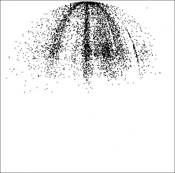
[Figure 1] Edge-on view (0-1) of the Universe through the space distribution of the BH quasar catalogue, by assuming a positive curvature $k_0=0.4$. The whole Universe is projected on to a unitary disc, and the Galaxy is located at the top edge, where the number density is the highest. The bottom edge of the distribution corresponds to a redshift $z\approx 4$, which shows that the sample of all known quasars fills, in space, slightly more than the half of the Universe (the unitary disc is not drawn). There is a lack of sources along the edge of the unitary disc owing to selection effects in observation which corresponds to the obscuration zone of the galactic plane. Similarly the structures along ellipses are a result of selection effects which depend on the line of sight. The horizontal structures (along chords) are a result of selection effects on redshift.

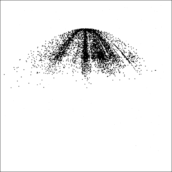
[Figure 2] Edge-on view (0-1) of the Universe, by assuming a negative curvature $k_0=-0.8$. The space distribution of the BH quasar catalogue is projected within a unitary hyperbola up to redshift $z\approx 4$. The lack of sources along the edge of the hyperbola is owing to the zone of avoidance in the Galactic plane.

4.1.2 Face-on views

In the face-on views [views $(i-j{)}_{0<i<j\le 3}$], the Galaxy is located at (0,0), the centre of the diagram, and the quasar distribution lies within a disc; see Figs 3 and 4. The pencil beams are projected on to radii, which defines the shape of related bogus structures owing to selection effects on the line of sight. The vertical zone of avoidance is caused by the obscuration of the Galactic plane. Let us mention that the bogus structures owing to redshift selection effects cannot be recognized in these maps ^[7]. While these projections offer fewer possibilities than the edge-on views for the identification of selection effects, they provide us with complementary information.

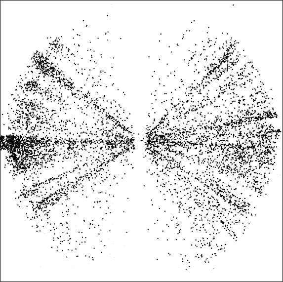
[Figure 3] Face-on view (1-2) of the Universe through the space distribution of the BH quasar catalogue, assuming ${\mathrm{\Omega }}_0=0.2$ and ${\lambda }_0=1.2$.

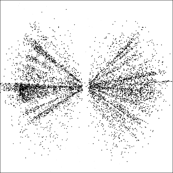
[Figure 4] Face-on view (1-2) of the Universe through the space distribution of the BH quasar catalogue, assuming ${\mathrm{\Omega }}_0=0.2$ and ${\lambda }_0=0$.

4.2 About the distortion problem

The main problem for visual analysis is related to the distortion effect (e.g., as in maps of the world). To investigate such a problem we have to calculate the image of the volume element on ${\hat{V}}_3$ using the above projections. It turns out that the volume element $dV$ can be written as follows:

$$\begin{array}{}\text{(38)}& dV=d(\cos \nu )d\varphi \times \{\begin{array}{ll}{\sin }^2(\hat{\tau })d\hat{\tau }& \text{if }{k}_0>0\\ {\sinh }^2(\hat{\tau })d\hat{\tau }& \text{if }{k}_0<0,\end{array}\end{array}$$

where $\nu$ is the angle defined by $⟨x,p_3{⟩}_3=\cos \nu$. Hence, it is obvious that the image reads $dudv$. Indeed, for the edge-on view, the Jacobian of the transformation of variables $(\hat{\tau },\cos \nu )\to (u,v)$ reads

$$\begin{array}{}\text{(39)}& J[(\hat{\tau },\cos \nu )\to (u,v)]=\{\begin{array}{ll}{\sin }^{-2}(\hat{\tau })& \text{if }{k}_0>0\\ {\sinh }^{-2}(\hat{\tau })& \text{if }{k}_0<0,\end{array}\end{array}$$

and the volume element may thus be transformed using $dV=dudvd\varphi$. Hence, the integration over $\varphi$ provides us with $dudv$, the image of the volume element on the map ^[8]. The face-on view shows the same advantage. Indeed, the case $k_0>0$ is obvious, for symmetry reasons, while for $k_0<0$ we use the variable transformation $[\hat{\tau },u=\sinh (\hat{\tau })\cos (v),v=\sinh (\hat{\tau })\cos (\varphi )]\to (\hat{\tau },v,\varphi )$ the Jacobian is equal to ${\sinh }^{-2}(\hat{\tau })$. Therefore, we understood that the shapes of LSSs are preserved ^[9] in the projections which provide us with the above maps, which ensures that the structures that can be seen on these maps do not correspond to artefacts.

5 CONCLUSION

This paper introduces an efficient geometrical framework for the investigation of large-scale structures at high redshift in curved spaces. The world models are given by Friedmann-Lemaitre models of Universe. This framework is implemented in a free-share routine (Universe Viewer) developed on a Unix station, which is available on the internet network at node cpt.univ-mrs.fr/cosmology/UV.

ACKNOWLEDGEMENTS

We thank Andrew Laycock for useful comments on the manuscript.

REFERENCES

• Bigot G., Triay R., 1990, Phys. Lett. A, 150, 227
• Burbidge G., Hewitt A., 1993, ApJS, 87, 451 (BH)
• Carroll S. M., Press W. H., Turner E. L., 1992, ARA&A, 30, 499
• Fliche H. H., Souriau J. M., Triay R., 1982, A&A, 108, 256
• Gliner E. B., 1965, Sov. Phys. JETP, 22, 378
• Linde A. D., 1982, Phys. Lett. B, 108, 389
• Peebles P. J. E., 1993, Principles of Physical Cosmology. Princeton Univ. Press, Princeton
• Pierce M. J., Welch D. L., McClure R. D., Van den Bergh S., Racine R., Stetson P. B., 1994, Nat, 371, 385
• Souriau J. M., 1974, in Colloques Internationaux du CNRS, 237, 59
• Souriau J. M., Triay R., 1995, Phys. Rev. D, submitted
• Triay R., 1981, thèse 3ème cycle, Université de Provence, Provence
• Van den Bergh D. A., 1991, in PASP Conf. Ser. 13, The formation and the Evolution of Star Clusters. Astron. Soc. Pac., San Francisco, p. 183
• Weinberg S., 1972, Gravitation and Cosmology. John Wiley & Sons, New York
• Wilkinson D., 1991, in Blanchard A., Celnikier L., Lachièze-Rey M., Trân Thanh Vân J., eds, Rencontres de Blois 1990, Physical Cosmology - Proc. 25th anniversary of the Cosmic Background Radiation Discovery. Editions Frontières, Gif sur Yvette, p. 97

---

1. The European Cosmological Network ↩︎

2. E-mail: triay@cpt.univ-mrs.fr ↩︎

3. Stage Informatique du DEA de Physique Théorique 94/95 ↩︎

4. To avoid confusion with notations given in the literature, let us write the RW metric as follows:

   $$d{s}^2=d{t}^2-R^2(t)[\frac{d{\chi }^2}{1-\kappa {\chi }^2}+{\chi }^2(d{\theta }^2+{\sin }^2\theta d{\varphi }^2)]$$

   where $\kappa =k_0|k_0{|}^{-1}$ is the sign of the curvature, and if it is not zero then $a(t)=R(t)H_0^{-1}|k_0{|}^{1/2}$, otherwise $a(t)=R(t)H_0^{-1}$ and finally one has the radial coordinate

   $$\chi =\{\begin{array}{ll}\sin \hat{\tau }& \text{if }{k}_0>0\\ \tau & \text{if }{k}_0=0\\ \sinh \hat{\tau }& \text{if }{k}_0<0.\end{array}$$ ↩︎

5. For example, $p_3$ ($RA=\alpha$, $Dec.=\delta$), $p_1$ is given by a rotation of angle $\psi$ about $p_3$ of a unitary vector $\propto e_3\times p_3$, and $p_2=p_3\times p_1$. ↩︎

6. Indeed, the first one is related to surveys sampling, such as pencil beams, ..., when the second is based on spectroscopic criteria, such as the chromatic sensitivity of receivers, ... The identification of main emission lines Mg II, Ly $\alpha$ N v, C III, C IV, Si IV, ... is possible when they lie within the observable wavelength range. ↩︎

7. Indeed, a region of the Universe at redshift $z$ is projected within a disc of radius given by $\sin \hat{\tau }(z)$ if $k_0>0$ or $\sinh \hat{\tau }(z)$ if $k_0<0$, which does not indicate the distance. ↩︎

8. Applied to the case of $S^2$ sphere projected on to a diameter (one-dimensional disc), it is a well-known theorem. ↩︎

9. In other words, the image of the uniform measure on ${\hat{V}}_3$ is still uniform. ↩︎